MHN Object Grouping
MHN Visual Representation
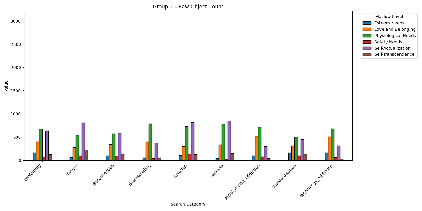
Raw Count
Each object is counted as 1, regardless of which image or category it appears in.
| Strengths: | Limitations: |
|
Preserves the real quantity of detected objects. Shows actual distribution of psychological content. |
Skewed by unequal category size and dense tagging in some images. Overrepresents categories with more images or complex scenes. |

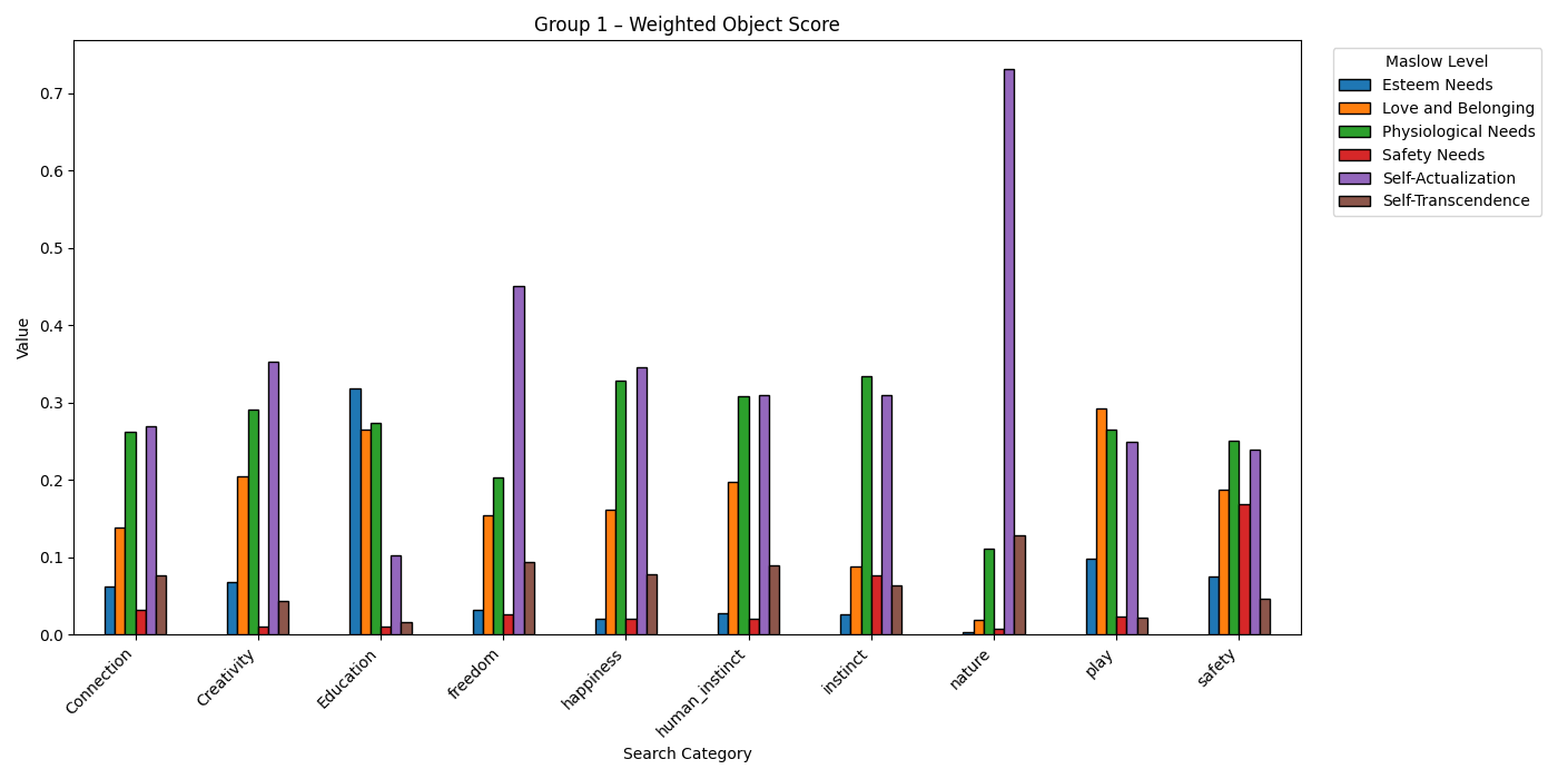
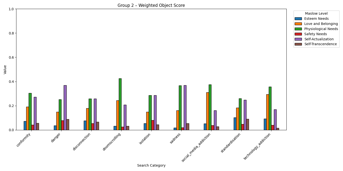
Weighted Count
Each object is assigned a weight:
w = (1 ÷ number of images in category) × (1 ÷ number of objects in its image)
| Strengths: | Limitations: |
|
Controls for category size and object density. Levels the playing field across uneven dataset structure. |
Reduces the impact of categories with genuinely more data. Still reflects absolute volume, not relative psychological emphasis. |
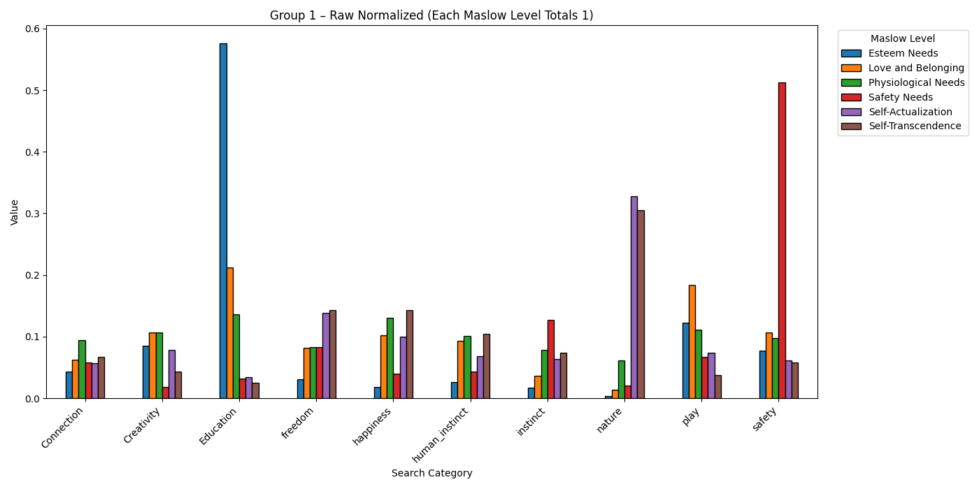
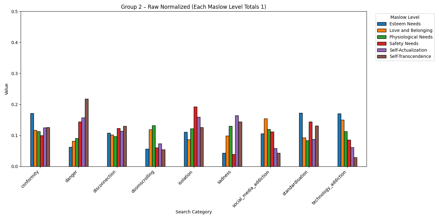
Raw Normalised
Same as Raw Count, but each Maslow level column is scaled to sum to 1.
| Strengths: | Limitations: |
|
Allowsproportional comparison of categories within each Maslow level. Reveals which categories dominate each psychological need. |
Still subject to category size bias. Doesn’t correct for object over-tagging in individual images. |
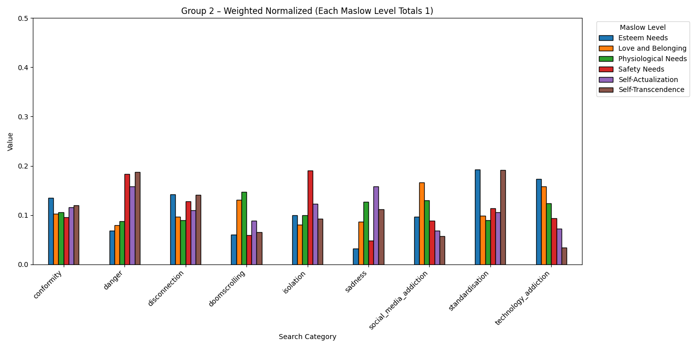
Weighted Normalised
Uses weighted object values
w = (1 ÷ category count) × (1 ÷ object count in image)
Then normalises each Maslow level column to sum to 1.0.
| Strengths: | Limitations: |
|
Controls for both category imbalance and object density. Best for analysing the relative psychological tone of each category. |
Creates a counterfactual model: assumes all categories are equally valid sources of meaning. May obscure real-world dominance or suppression of certain needs. |